Running the WRF model is very easy: just find a good computer, follow the tutorials, compile and run. The real challenge is creating meaningful numerical experiments and critically evaluating the model output.
Introduction
A typical atmospheric modeling class (hereafter ATMMOD) involves reviewing topics from different subjects in upper-level undergraduate and graduate level meteorology and atmospheric sciences. My atmospheric modeling class (now in its fifth version in English and third version in Spanish) includes basic elements of atmospheric physics as they relate to atmospheric modeling (e.g. Stensrud 2007). However, since my first lecture, I made it a point to also include hands-on work with a real atmospheric model such as the Weather and Research Forecasting model (WRF; Skamarock et al. 2008).
My original goal was to offer give a class that not only teaches how to effectively use one of the most popular and state-of-the-art atmospheric models, but also provides the elements for the understanding of processes and interactions in the atmosphere. However, there are numerous limitations, challenges, rewarding anecdotes and frustrating situations that I believe are worth sharing in this article.
Why WRF?
Balancing the theoretical and practical (if any) components of a modeling class can be challenging. Syllabi tend to be general and include theory and concepts that are common across climate system components (water and ice, biology and ecosystems, and atmosphere), model hierarchy and spatio-temporal scales. The model hierarchies and complexity vary from Earth Systems and Global Climate Models (GCM; 106–105 m) to regional climate or mesoscale models (105 – 103 m) to computation fluid dynamic models (~102 – 1 m).
A common component of the atmospheric models, regardless of the scale, is the system of equations that govern the fluid dynamics –the Navier-Stokes (N-S) system of equations. However, some adaptations are often needed as some forces are negligible according to the scale of motion implemented. The numerical solutions for the integration of the N-S equations can also change based on scale and model complexity.
Some significant differences across models are found in the treatment and parameterization of radiation, moist processes, turbulence, and transport of mass in the atmosphere (Maher et al. 2019). Students in a classroom setting need to be aware of both the theory and the practical consequences of these differences.
The hands-on portion of an ATMMOD class often teaches how to develop simple and low-dimensional models –with adequate assumptions and idealized domains–, while others include learning and practicing with more realistic tools. For example, the EdGCM (Chandler et al. 2005; http://edgcm.columbia.edu/) was developed to bring a GCM (with a 5º grid size) into the classroom and make it easy for the educator and the students in academic setups. I have personally used it in the past for my ATMMOD class. I enjoyed the tool and was very insightful for the students. Even though EdGCM serves its academic purpose, and it constitutes a tool for research-grade GCM solutions, I would argue that it focuses a bit too much towards climate projections and climate sensitivities; EdGCM doesn’t resolve many physical phenomena of scientific and practical interest, i.e., great for general circulation related features but too coarse for storms, hurricanes, atmospheric rivers, etc.
My ATMMOD class has evolved to include just enough theory and a rather busy hands-on component. I have opted to be somewhere in the middle of scales and model hierarchy for the hands-on component, focusing on how to use the mesoscale model WRF. This is partly due to the fact that I have been using WRF in my research since 2004, and it is the model I am most familiar with. Furthermore, is freely available WRF and is one of the most popular atmospheric models with thousands of users (more than 30000 according to Wikipedia as of April 2020). It is a community model developed by multiple agencies and maintained by NCAR since 2000 (https://www.mmm.ucar.edu/weather-research-and-forecasting-model). Among the users are weather forecasting agencies, universities and government, and private companies.
The model applications for WRF keep growing, involving areas that span numerical weather forecasting, regional climate modeling –analysis and future projections–, dispersion and air quality, fire and atmospheric chemistry, hydrology, agriculture, energy and renewables, earth systems modeling, among other applications (Powers et al. 2017). Extensive use of such models demands educating the work force to accelerate their learning. It also demands we as educators provide basic guidelines for adequate reasoning and conscious use of modeling tools (Curry and Webster 2011; Warner 2011).
NCAR regularly offers onsite WRF training courses and webinars (https://www.mmm.ucar.edu/wrf-tutorial-0). Nevertheless, bringing WRF to the ATMMOD classroom can be a great opportunity to extend the mission of the atmospheric science community while, at the same time, contribute to reach out to more students (Steeneveld and Vilà-Guerau de Arellano 2019).
Desirable Prerequisites
Ideally, one would like to teach an ATMMOD class to students who are familiar with atmospheric physics, numerical methods (interpolation, integration, differentiation, etc.), who have ample knowledge about environmental and remote sensing datasets from different platforms and formats, and who have experience with tools that facilitate model output manipulation and visualization. Additionally, I consider a bonus having enrolled students with scientific computing skills, including familiarity with Linux environment, basic programming (e.g., Python, MATLAB, Fortran), high-performance computing and cluster operations, Big Data manipulation, and statistics and analytics tools.
However, it is hard to find students that will satisfy all these prerequisites. The reality is that many of our geosciences and physics programs often teach atmospheric or environmental modeling courses, with students that tend to be trained in multidisciplinary and interdisciplinary undergraduate degrees. Fortunately, at graduate level, students tend to satisfy many of the elements listed above, making the class easier for both teacher and students. For a few students, it can be a steep learning curve, but again, one has to start from somewhere.
Compiling and porting WRF code to a specific machine or cluster can be a very challenging and often frustrating task. To minimize delays in the class with that particular issue, I strongly avoid teaching how to install the model. Instead, I provide ready-to-use, compiled code that I have already tested. Hacker et al. (2017) showed the advantage of including a “containerized WRF” for classroom and research activities, which eliminates the compiling and porting delays, and is multiplatform (Linux, Mac, Windows). Adapting to this containerized WRF option sounds advantageous, but still requires some additional knowledge for new users and seems to be a paradigm shift for the old ones.
I have been fortunate to have high-performance computing (HPC) systems available for my classes. During summer 2015, I taught the ATMMOD class (Spanish version) at the National University of Colombia, at Medellin (UNALMED). More than 20 upper-level undergraduate and graduate students were enrolled from various universities in the region, including Air Force and Navy research and operational personnel (sponsored by COLCIENCIAS; https://minciencias.gov.co/).
I teach the English version of ATMMOD every two years for the Atmospheric Science graduate program at the University of Nevada, Reno. We typically have a dozen students per class. Computing for the hands-on component is provided by the Desert Research Institute, which also facilitates a dedicated cluster for our graduate research assistants.
Lab component
One interesting and fun aspect of the hands-on component of the class is that one can attempt to simulate atmospheric phenomena that are of interest to the students. During the ATMMOD class in summer 2015 in Colombia, the students were intrigued about whether the model was skillful in simulating Tropical Easterly Wave incursions over the Caribbean Sea, and moreover, if it could capture their impacts on precipitation over the Colombian Andes. I designed a simulation of a 10-day long period in which each student (24 students) got to simulate that scenario using different physics model configuration, including different parameterization options. The result was something akin to a classroom “poor-man’s” ensemble.
All simulations were submitted during the class on Thursday morning, and all model output were ready by the end of the weekend. During the following class, I distributed Python scripts designed to extract simulated surface model parameters and develop basic output visualization. In the lab, students also learned how to evaluate the model output using point precipitation measurements and gridded data.
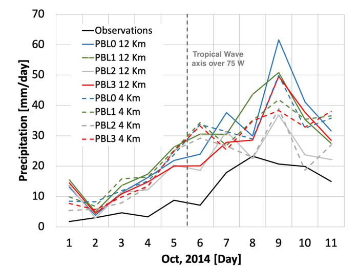
Figure 1 shows one example highlighting the sensitivity of the simulated precipitation to four widely used PBL parameterization schemes (local and non-local) and for two nested domains (12 km and 4 km grid sizes). Similar analysis (not shown) were explored for sensitivity around other processes, while introducing concepts regarding suitability (or lack thereof) of physics-based ensembles, and scale dependence.
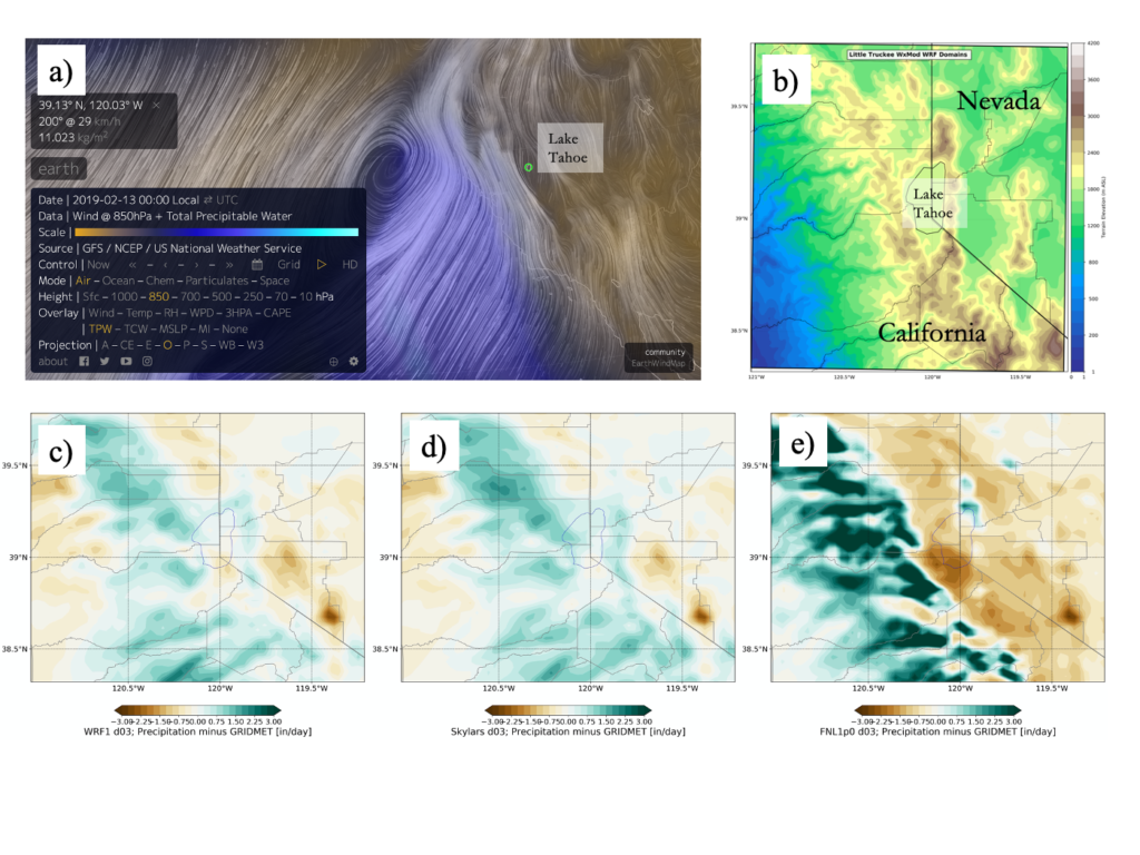
More recently, during the ATMMOD class of fall 2019 I taught at the University of Nevada at Reno, my students dedicated the hands-on activities to study the simulated precipitation related to a landfalling Atmospheric River as it impacted northern California and the Sierra Nevada. I designed the lab component of the class to test sensitivity to different parameterization options and different used initial/boundary conditions datasets, with particular emphasis on cloud resolving scales (grid sizes of 4km and smaller and turning off convection parameterization.
I showed Figure 2 in class to discuss the sensitivity to different microphysics schemes precipitation biases. However, the students noticed that precipitation was more sensitive to the use of different initial/boundary conditions datasets than to the microphysics. Results enable discussion on how the model was overdoing the orographic forcing, regardless of the physical setup.
Although these class activities are interesting but far to deliver a generalized conclusion, they can have important operational and research implications. Nevertheless, the in-class discussions included exciting elements of sources of uncertainty and how model sensitivity to various parameters often allude to exercises designed for model “tune up” or “calibration”, terms that I try to avoid using in model sensitivity studies. Instead, I suggest that short-term studies should be used with caution and that the decision of implementing a single set of parameterization option is challenging as the error structures are flow- and season-dependent (García‐Díez et al. 2013).
The course culminates in a term project that includes designing their own model simulation around a research idea or an atmospheric process of their interest. For this term project, students can opt to examine more deeply the model output of the exercises developed during the hand-on activities.
Closing remarks
The original goals associated with this course were to provide upper-level undergraduate and graduate students with up-to-date, practical and skillful knowledge of atmospheric modeling, including modeling analysis and a handful of analytic metrics and tools. The ultimate goal is for students to use their critical thinking skills, while learning basic concepts of model uncertainty, prediction skill, predictability and deterministic and ensemble modeling solutions.
This course has been a jump start for the research work of many graduate students. It has definitely provided arguably some needed exposure to WRF, from start to end (except installation procedures).
High-performance computing facilities are increasingly available and the WRF model is becoming more widely implemented in various impact areas. Hence, there is a pressing need for students to have some exposure to the model. There are many challenges associated with the introduction of the WRF model in a class setting as many prerequisites are desirable in order to have a smooth learning process. Students can often feel overwhelmed by the models’ complexity. Course enrolment is typically limited by computer lab capacity.
This article constitutes my opinion and it highlights the situations, benefits, limitations on the processes I have learned from running WRF in my atmospheric modeling class. It does not provide elements necessary to be a good teacher and does not make a new or old modeler a good modeler (Warner 2011). Definitely, it is not a unique experience as other have successfully taught complex modeling tools in the classroom (Chandler et al. 2005, Steeneveld and Vilà-Guerau de Arellano 2019; Hacker et al. 2017).
WRF is here to stay likely due to the pressing demand of incorporating detailed weather and climate diagnostic and prognostic information in the decision-making process, fundamentally in all production and commerce enterprises, as well as in water, energy, ecosystem- and food-resource management (Powers et al. 2017).
This text may also be of interest in other academic settings that attempt to build a bridge between theory and models or other computational analytical tools. And note that NCAR/CISL (https://www2.cisl.ucar.edu/user-support/allocations/university-allocations#classroom) offers HPC education allocations for classes that require hand-on simulations.
Acknowledgments: Thanks to all the students that contributed to make this class a rewarding teaching experience. Thanks to Drs. Benjamin Hatchett, Juan Jose Henao, and Bradford Barrett for their insightful comments and suggestions. NSF-EPSCoR, DRI/UNR, COLCIENCIAS and UNALMED have contributed funding and in-kind resources to develop this class.
References
Chandler, M.A., S.J. Richards, and M.J. Shopsin, 2005: EdGCM: Enhancing climate science education through climate modeling research projects. In Proceedings of the 85th Annual Meeting of the American Meteorological Society, 14th Symposium on Education, Jan 8-14, 2005, San Diego, CA, pp. P1.5. http://edgcm.columbia.edu
Curry, J. A., & Webster, P. J., 2011: Climate science and the uncertainty monster. Bull. Amer. Meteor. Soc., 92(12), 1667-1682.
García‐Díez, M., Fernández, J., Fita, L. and Yagüe, C., 2013: Seasonal dependence of WRF model biases and sensitivity to PBL schemes over Europe. Q.J.R. Meteorol. Soc., 139: 501-514. doi:10.1002/qj.1976
Hacker, Joshua P., John Exby, David Gill, Ivo Jimenez, Carlos Maltzahn, Timothy See, Gretchen Mullendore, and Kathryn Fossell, 2017: A containerized mesoscale model and analysis toolkit to accelerate classroom learning, collaborative research, and uncertainty quantification. Bull. Amer. Meteor. Soc., 98, no. 6, 1129-1138.
Maher, P., Gerber, E. P., Medeiros, B., Merlis, T. M., Sherwood, S., Sheshadri, A., et al., 2019: Model hierarchies for understanding atmospheric circulation, Reviews of Geophysics, 57, 250– 280. https://doi.org/10.1029/2018RG000607
Powers, J.G., J.B. Klemp, W.C. Skamarock, C.A. Davis, J. Dudhia, D.O. Gill, J.L. Coen, D.J. Gochis, R. Ahmadov, S.E. Peckham, G.A. Grell, J. Michalakes, S. Trahan, S.G. Benjamin, C.R. Alexander, G.J. Dimego, W. Wang, C.S. Schwartz, G.S. Romine, Z. Liu, C. Snyder, F. Chen, M.J. Barlage, W. Yu, and M.G. Duda, 2017: The Weather Research and Forecasting Model: Overview, System Efforts, and Future Directions. Bull. Amer. Meteor. Soc., 98, 1717–1737, https://doi.org/10.1175/BAMS-D-15-00308.1
Skamarock, W. C., J. B. Klemp, J. Dudhia, D. O. Gill, D. M. Barker, M. G Duda, X.-Y. Huang, W. Wang, and J. G. Powers, 2008: A Description of the Advanced Research WRF Version 3. NCAR Tech. Note NCAR/TN-475+STR, 113 pp.
doi:10.5065/D68S4MVH
Steeneveld, G. and J. Vilà-Guerau de Arellano, 2019: Teaching Atmospheric Modeling at the Graduate Level: 15 Years of Using Mesoscale Models as Educational Tools in an Active Learning Environment. Bull. Amer. Meteor. Soc., 100, 2157–2174, https://doi.org/10.1175/BAMS-D-17-0166.1
Stensrud, David J., 2007: Parameterization Schemes: Keys to Understanding Numerical Weather Prediction Models, Cambridge University Press, DOI:https://doi.org/10.1017/CBO9780511812590
Warner, T. T. (2011). Quality assurance in atmospheric modeling. Bull. Amer. Meteor. Soc., 92(12), 1601-1610.
Dr. Mejia is an Associate Research Professor in the Division of Atmospheric Sciences, Desert Research Institute and a professor for the Atmospheric Science Graduate program, University of Nevada, Reno, NV. His research is closely related to observing, understanding, and modeling weather and climate at different spatial and temporal scales. When he is not coding and running models, you will find him developing outreach and education relationships in the U.S. and Latin American.